beavers Who are Busy

This post is going to discuss one of the many ways that data scientists tame data to allow supervised image processing models to handle weirder looking images and generally perform better.

The way this is done is through the application of some kind of filter to the image you want to classify (or identify, or all the other stuff you might wanna do), before it is fed to the algorithm.

There are many different types of filters that may be applied, and the exact choise of filter(s) will depend on the task, but the one we will cover today will be gaussian noise (we’ll be doing gaussian blur next week).

Gaussian Noise:

Gaussian noise is often used to deal with the task of having to identify features within a potentially static-ey image. For example you may have a training dataset for your model that has basically no static, but you might want to to able to identify static-ey images. In order to ensure that your model performs well on both static-ey and non-static-ey images, you can just make sure that every input is static-ey, and not worry about differentiating them.

So how can you make sure everything has static? Well you can just add it in using the ideas of gaussian noise as a preliminary step for your algorithm (It would take in the image, add static to it, then run the model on the static-ey image).

But how does gaussian static actually work? And why is it called that?

Well one way of thinking about it is to imagine that you are making a sheet of randomly colored pixels and laying it in top of your original image. This sheet can be generated using a gaussian distribution, which has the equation e^(x^2) and looks like this:

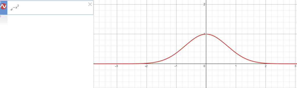
(There are some other fancy terms you can add, but this is enough for this investigation)

Basically, the values we can choose for each pixel of our sheet are represented by the values along the x axis, and the chance that we choose any individual x-value for a pixel is represented by its correspondent y value in the gaussian. Practically, since RGB values only range from 0 to 255, we won’t use the whole distribution when we implement this on a computer.

In order to randomly choose from this distribution while abiding by the probabilities it assigns to each possible x value, we choose a random real number on the interval (-1,1) (where every single number is equally likely to be chosen) and take it as an input to the inverse of something called the error function. We can represent this in the computer as

gaussian_choice(): return erfinv(random.uniform(-1,1)).

We can run the gaussian_choice() function for every pixel of our overlay sheet, and add the resultant values to the original image, getting a more static-ey version.

Why we use the inverse of the error function:

The error function is defined as

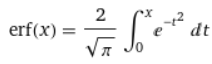
Basically, it’s the area under the gaussian curve from x=-X to x=X, where big X is the input.

In order to choose every possible x value with the proper probability density, we would like a function that satisfies the differential equation

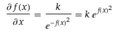
Where k is some constant we don’t actually care about (we’ll decide what it is later, so that the end result is most convenient). The basic idea behind why we want it to satisfy this equation is that we would like the outputs of f(x) to correspond to positions on the x-axis for the actual gaussian function, and we want it to slow down at places where the correspondent probability is high. There’s a bit more detail to get into on this point, but this post is getting long (and my hands are getting tired), so I’ll leave that as homework for anyone who wants to do it.

Solving the differential equation you’ll get that

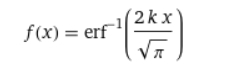
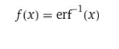
here we can decide that k was sqrt(pi)/2 the whole time, and it becomes

The main reason why I wanted to share this idea with you all is because its a great example of how math can make for a slicker algorithm, and how a specific problem can sometimes be rephrased in terms of more general ones. Hopefully, the way that we turned the complex problem of selecting values from a nonuniform distribution into a combination of the problems of selection from a uniform distribution and apporoximation of the inverse error function can serve as inspiration for you in the future, when you are looking for ways of developing 1-dimensional solutions to problems that exist in multiple dimensions.